2. Mechanics

2.1. Introduction

All man-made constructions (but also all natural structures) are under the influence of forces, temperature changes and vibrations. Sometimes such loads are constantly present and predictable, sometimes they occur sporadically and have a casual character.

A structure will deform as a result of loads. Excessive deformations can hamper functioning and lead to damage in the form of excessive wear and even breakage. When designing a structure, care must be taken that occurring deformations are small enough to ensure reliable operation and a sufficiently long service life. Predicting deformation caused by stress occurs with the help of theories and techniques from mechanics. It is essential here that people know how the material of which the construction is made behaves. This material behavior can be measured in a laboratory and then described with a material model.

A few concepts from mechanics will be introduced in this chapter. Furthermore, we will describe the material behavior of a typical steel type. Finally, we will see that for practical problems the use of computers and software is essential for predicting the mechanical behavior of a structure.

2.2. The rod: a one-dimensional construction element

In many constructions, machines and structures we can recognize parts that we can regard as a rod: a slender (long in one direction and short in the other directions) part that transmits a force in its longitudinal direction (= axial).

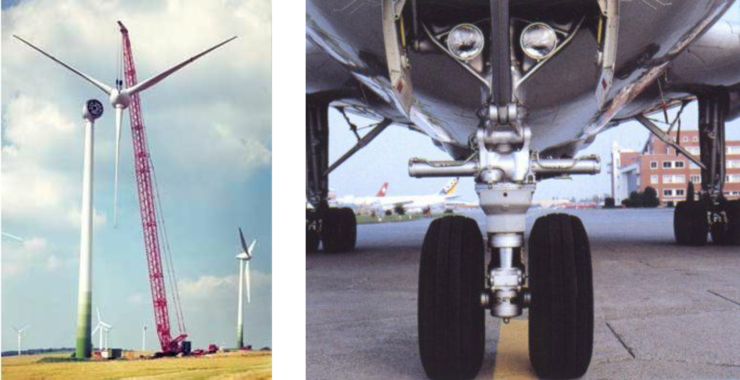
Fig. 2.1 Constructions with axially loaded parts.

The mechanical behavior of such a rod can be studied in the laboratory. A test is carried out with the aid of a tensile tester in which the rod is loaded in its longitudinal direction. The change in length due to the axial load is measured. We assume that the tensile bar in its initial condition has a length \(L_0\) and a cylindrical cross-section with surface \(A_0\). When the tensile bar is subjected to tensile load by an axial force F, the length will increase by \(L\) as outlined in Fig. 2.2 below.

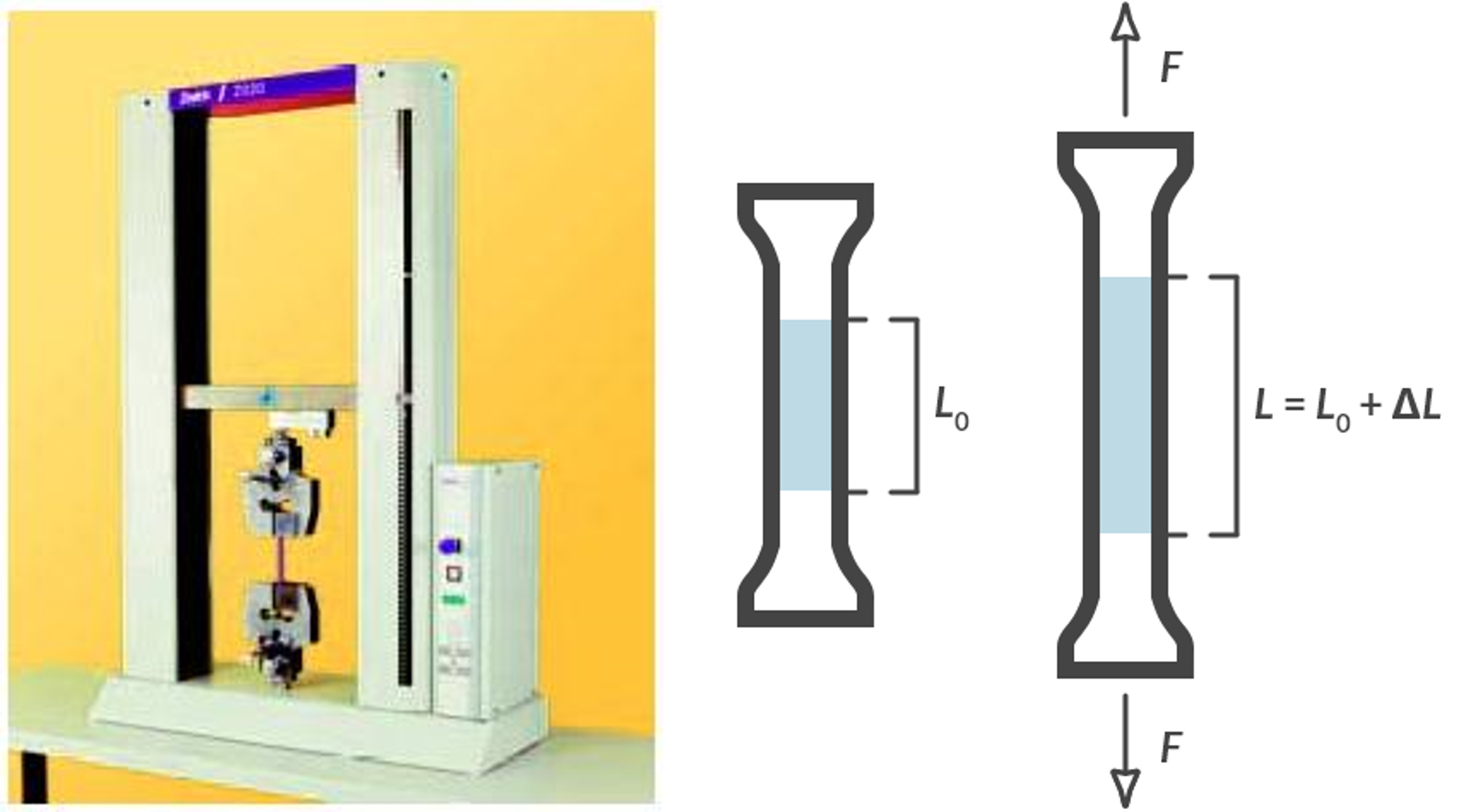
Fig. 2.2 (a) Tensile tester (source: Zwick), (b) tensile bar under load of a force \(F\).

If the extension is small, the relationship between \(F\) and \(\Delta L\) will be linear, therefore we can state:

(2.1)\[ F = k \cdot \Delta L \]

The proportionality factor \(k\) is called the stiffness of the bar. Experimentally it appears that the stiffness is proportional to the area of the cross-section \(A_0\) and inversely proportional to the length \(L_0\):

(2.2)\[ F = k(A_0, L_0) \cdot \Delta L \text{ with } k \propto A_0 \text{ and } k \propto \frac{1}{L_0} \to F = \frac{E \cdot A_0}{L_0} \cdot \Delta L\]

The parameter \(E\) appears to depend only on the material from which the bar is made and not on its dimensions. This material parameter is the elastic modulus.

By rewriting the above relationship, we see that the modulus of elasticity describes the linear relationship between and . These quantities play an important role. It is the nominal stress \(\sigma_n\) and the linear strain \(e\).

(2.3)\[ \frac{F}{A_0} = E \cdot \frac{\Delta L}{L_0} \to \sigma_n = E \cdot e\]

The linear relationship between \(\sigma_n\) and \(e\) indicates linear elastic material behavior and is known as Hooke’s Law. The word elastic indicates that, after the axial force has been removed, no permanent deformation of the rod can be measured: its length is again \(L_0\). Check this yourself.

Do you know the answer to the following question?

Robert Hooke (1635-1703) [1]

Robert Hooke FRS (18 July 1635 – 3 March 1703) was an English physicist (“natural philosopher”), astronomer, geologist, meteorologist and architect. He is credited as one of the first scientists to investigate living things at microscopic scale in 1665, using a compound microscope that he designed. Hooke was an impoverished scientific inquirer in young adulthood who went on to became one of the most important scientists of his time.[8] After the Great Fire of London in 1666, Hooke (as a surveyor and architect) attained wealth and esteem by performing more than half of the property line surveys and assisting with the city’s rapid reconstruction. Often vilified by writers in the centuries after his death, his reputation was restored at the end of the twentieth century and he has been called “England’s Leonardo [da Vinci]”.

Fig. 2.3 Portrait of Robert Hooke.

With a tensile tester we can also exert an axial pressure on the rod. According to agreement, the tension in the rod is then negative and that also applies to the strain that describes the shortening of the bar. For small negative strains, the relationship between n and \(e\) is described for almost all materials by the same elastic modulus \(E\) that we determined during the tensile test. We say that the linear elastic material behavior for tensile and pressure is identical.

If the length of the bar becomes longer or shorter during a tensile or compression test, the cross-sectional area will also change. It is clear that the bar becomes thinner with extension and thicker with shortening. For a rod with a circular cross section, we can indicate the thickness change with the diameter change \(\Delta D\). We can then introduce a new strain, the transverse strain ed,

(2.4)\[ e_d = \frac{\Delta D}{D_0}\]

With \(D_0\) the diameter of the undeformed rod. By accurately measuring the change in diameter, which is extremely small, during the tensile/pressure test, it appears that for linear elastic material behavior the following relationship exists between the transverse strain and the axial strain:

(2.5)\[ e_d = -v \cdot e\]

The material parameter \(v\) is called the Poisson ratio and is independent of the shape of the cross-section.

Elongation of a rod

A tensile force of 40000 N is applied to an aluminum rod with a diameter of 1.0 cm and a length of 2.0 meters. How far does the bar stretch? How much does the bar become thinner? See Table 2.1 for material data.

Solution

The following applies to the tension in the rod:

(2.6)\[ \sigma_n = \frac{F}{A_0} = \frac{F}{\frac{1}{4}\pi d_0^2} = \frac{40000}{\frac{1}{4}\pi (0.01)^2} = 5.09 \cdot 10^8 \textrm{ [Pa]} \]

With the modulus of elasticity of aluminum of 70 GPa the elongation becomes:

(2.7)\[ e = \frac{\sigma_n}{E} = \frac{5.09 \cdot 10^8}{70 \cdot 10^9} = 7.28 \cdot 10^{-3} \textrm{ [-]}\]

For a rod of \(2.0 \textrm{m}\) this gives an extension of: \(\Delta L = L_0 \cdot e = 2.0 \cdot 7.28 \cdot 10^{-3} = 1.46 \cdot 10^{-2} \textrm{m} = 1.46 \textrm{cm}\).

The transverse strain is equal to: \(e_d = -v e = 0.21 \times 7.28 \cdot 10^{-3} = -1.53 \cdot 10^{-3}\).

After elongation the rod is \(\Delta D = e_d \cdot D_0 = -1.53 \cdot 10^{-3} \times 1 \textrm{cm} = 1.53 \cdot 10^{-3} \textrm{cm}\) thinner.

2.3. The stress-strain curve

Instead of the force ( stress), we can also prescribe the length change ( strain) of the test bar with a tensile tester. If the bar is extended, we can then register the stress-strain curve below.

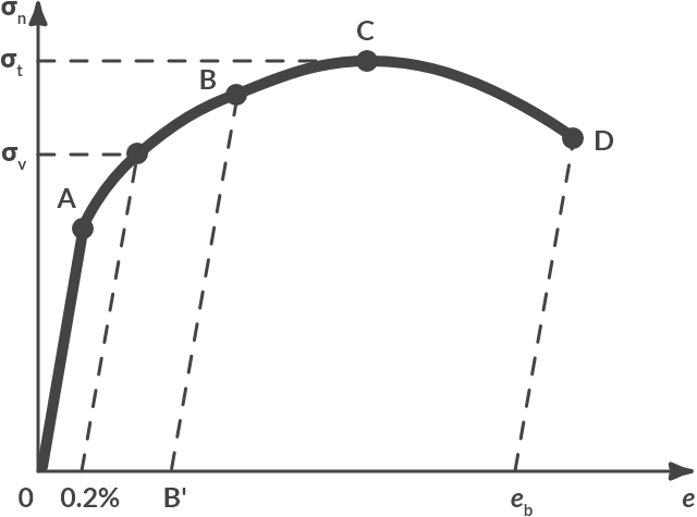
Fig. 2.4 Stress-strain curve for a typical steel alloy.

Up to point \(A\) there is linear elastic material behavior (\(\sigma_n = E \cdot e\)). From point \(A\), the relationship between \(\sigma_n\) and \(e\) is no longer linear. When in point \(B\) we let the tension become zero (= relieve), we can conclude that the test bar has undergone permanent extension: the material is plastically deformed.

When relieving pressure, the line \(BB\) ’is followed in the stress-strain curve, which turns out to be parallel to \(OA\). When loading again from point \(B\), we go up again past \(B’B\) until point \(B\) continues the initial stress-strain curve.

The stress at which the permanent (= plastic) elongation is 0.2% is called the yield stress of the material. Up to point \(C\), the stress increases with increasing elongation, a phenomenon called reinforcement. The maximum value of the stress that is reached in point \(C\) is the tensile strength \(\sigma_t\).

Upon reaching point \(C\), strange things happen to our test bar. The rod no longer remains nicely cylindrical but will start necking at a certain place, as can be seen in Fig. 2.5

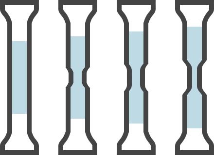
Fig. 2.5 Necking of a test bar.

In the neck, the cross-section will quickly become smaller with increasing elongation, while the other parts of the bar will hardly deform further. The tensile force \(F\) and the stress n will become smaller. In point \(D\), the rod is weakened by the increased neck so much that it breaks. The permanent plastic elongation after fracture is the fracture strain or elongation at break \(e_b\) .

The properties of materials can vary greatly. Table 2.1 shows the values of characteristic parameters for a few materials, which were determined by means of a tensile test and which were discussed above.

Table 2.1 Characteristic parameters for some materials.

Material	\(E\) [GPa]	\(v\) [-]	\(\sigma_v\) [MPa]	\(\sigma_t\) [MPa]	\(e_b\) [-]
Steel	210	0.3	200	650	0.1
Stainless steel (type 304)	193		205	515
Cast iron	110			310
Copper	105			455
Aluminium (99.9%)	70	0.21		125	0.4
Titanium	110
Carbon fiber	230			3,800 - 4,200
Optical fiber	72.5	0.22		1,020
Polypropylene (PP)	1.14 - 1.55
Polyethylene (PET)	2.76 - 4.14		59	48.3 - 72.4
Polyvinylchloride (PVC)	2.14 - 4.14	0.38	40.7 - 44.8	40.7 - 51.7
Nylon 6.6	1.59 - 3.79	0.39
Rubber		0.5
Wood	12		108

The major differences in properties can be explained by considering the atoms and molecules that make up the materials and the way in which these building blocks are arranged.

2.4. Maximum allowable stress

In practice, it will usually not be permissible for a rod to deform plastically. The tensile/compressive stress occurring in the rod must therefore remain lower than the yield stress \(\sigma_v\).

2.4.1. Danger 1: Buckling

When a thin rod is loaded with a compressive force, the yield stress \(\sigma_v\) may not be reached. As everyone knows from experience, a thin bar will buckle under pressure loading, which is accompanied by large lateral displacement of points of the bar, as shown in the figure below. The force at which buckling occurs is the buckling load \(F_k\). The value of \(F_k\) depends on the way the bar is supported, but also on the shape of the cross-section, characterized by the second moment of area \(I\). For a circular cross-section, the following applies: \(I = \pi \cdot D^4/64\) and for a square \( (h \times h): I = h^4/12\). Fig. 2.6 shows how a bar bends for different supports. Table 2.2 shows the corresponding values of the buckling force \(F_k\).

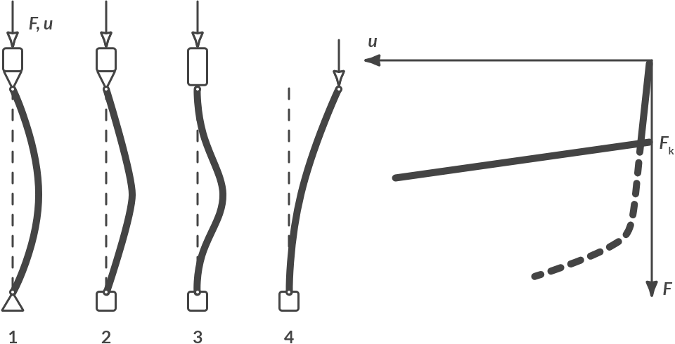
Fig. 2.6 Buckling with various supports of a rod.

Table 2.2 Buckling load for various supports.

	1	2	3	4
\(F_k\)	\(\dfrac{\pi^2 E I}{L_0^2}\)	\(\dfrac{\pi^2 E I}{(0.7L_0)^2}\)	\(\dfrac{\pi^2 E I}{(0.5L_0)^2}\)	\(\dfrac{\pi^2 E I}{(2L_0)^2}\)

In Table 2.2, \(L_0\) is the starting length of the rod. After the rod has buckled, the stiffness will be greatly reduced, as shown in the figure. If the displacement \(u\) is not too large, the material behavior remains elastic and the rod will regain its original length when the compressive force is removed. In practice however, it will often happen that the displacement becomes too large and the rod breaks. Because of this and due to the fact that \(F_k\) often has a low value, buckling is a dangerous phenomenon that must be taken into account during the design of rod structures.

2.4.2. Danger 2: Fatigue

When the bar is subject to a load whose magnitude varies with time, the bar breaks over time, although the maximum stress is lower than the yield or buckling stress. This phenomenon is called fatigue. Experimentally it can be determined for a certain material how large the number of load changes to fracture, \(N_f\), is at a certain stress amplitude \(\Delta \sigma\) By carrying out the experiment for different values of \(\Delta \sigma\) a so-called (S-N)-curve can be determined, where \(S\) stands for \(\Delta \sigma\). A typical (S-N) curve is shown in Fig. 2.7.

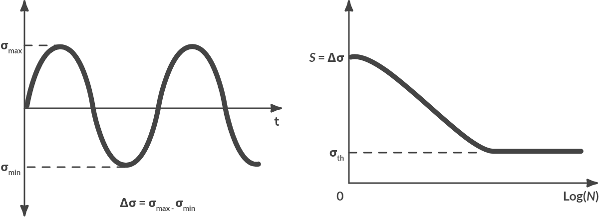
Fig. 2.7 Fluctuating stresses and (S-N)-curve (typical).

The number of load changes to breakage can be very large. For the drawn curve it is even the case that the lifetime becomes infinite when the stress amplitude remains below a limit value \(\sigma\)th. Fig. 2.8 shows the measured (S-N)-curves for several materials.

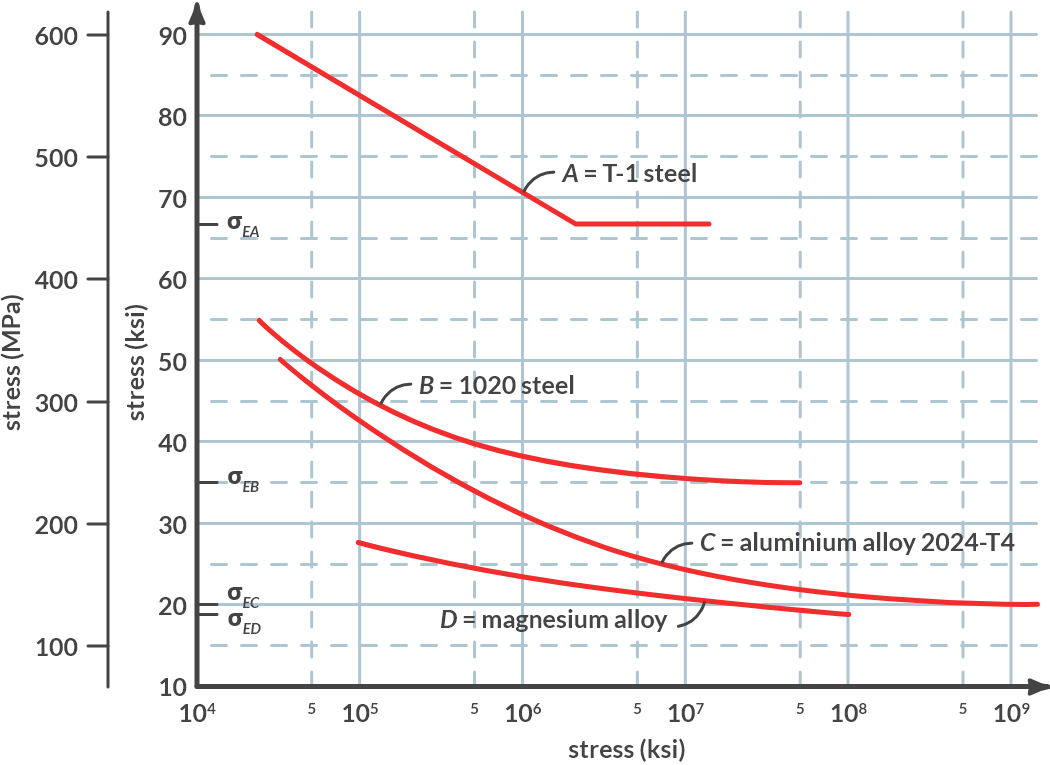
Fig. 2.8 (S-N)-curve for several materials.

Fortunately, such experimental data is readily available in the literature, so that we almost never have to perform such time-consuming experiments ourselves.

2.4.3. Safety factors

The calculation of deformations and stresses is based on mathematical models for equilibrium and material behavior. Model and material parameters must be determined through experiments. Results of model calculations and simulations cannot be fully trusted for the following reasons:

1. Simplifications in modeling. When formulating a model, reality is always simplified. As a result, no model will be able to describe reality with 100% accuracy.

2. Uncertainties in modeling. The properties of the materials from which a structure is constructed can differ from what is known or measured in a laboratory. Moreover, the measurement of material parameters is always done with finite accuracy.

3. Uncertainties in operating conditions. The (nature of) the actual load may be different from the load used for the calculations in the model. The conditions under which the structure must function can change the material properties.

Because of the uncertainties mentioned, safety margins are built in when designing structures. Calculation results are applied with a certain safety factor. Calculated limit values are adjusted downwards. The calculation models have improved considerably in recent years. More and more aspects of reality can be included in the modeling. This is mainly due to the considerably increased computing power of computers. The consequence of this is that the accuracy of the calculation results increases, and safety factors can decrease.

Bridge structure

Fig. 2.9 (a) shows a bridge truss structure that a small train (m = 2040 kg) must ride over. Fig. 2.9 (b) shows a schematic representation of this structure, for the situation where the train is in the middle of the bridge. The beams AB, BC, etc are all of the same length.

Fig. 2.9 (a) Construction of bridge with train (b) Schematic when train is in the middle.

For the situation where the train is in the middle of the bridge, the beam forces in the bridge have been calculated. These are given in the table below.

Table 2.3 Member forces in the truss structure of the bridge.

Member	\(F\) [kN]
AB	5.77
BC	5.77
CE	-11.55
DE	-20
AD	-11.55
BD	11.55
BE	11.55

The beams are connected to each other via pivot points. All beams are 6 meters long, have a round cross-section with a diameter of 0.05 meters and are made of steel.

1. Calculate the stress in each beam.

Solution

1. The stress in the beam can be calculated by \(\sigma F/A\). All bars have the same cross-sectional area \(A = \pi D^2 /4 = 1.96 \cdot 10^{-3} \textrm{m}^2\). The stresses thus become:

Table 2.4 Stresses in the beams.

Member	\(F\) [kN]	\(A\) [m\(^2\)]	\(\sigma\) [MPa]
AB	5.77	1.96 \(\cdot\) 10\(^{-3}\)	2.94
BC	5.77	1.96 \(\cdot\) 10\(^{-3}\)	2.94
CE	-11.55	1.96 \(\cdot\) 10\(^{-3}\)	-5.88
DE	-20	1.96 \(\cdot\) 10\(^{-3}\)	-10.19
AD	-11.55	1.96 \(\cdot\) 10\(^{-3}\)	-5.88
BD	11.55	1.96 \(\cdot\) 10\(^{-3}\)	5.88
BE	11.55	1.96 \(\cdot\) 10\(^{-3}\)	5.88

2. Is the maximum allowable tensile stress achieved in one of the beams?

Solution

2. The maximum tensile stress of steel is 200 MPa (see Table 2.1). This stress is not achieved in any of the elements.

3. Can this bridge bear the load? Explain!

Solution

3. Although the maximum tensile stress is not exceeded, there is a risk of buckling. As all bars are connected to each other via hinges, buckling variant 1 (see Fig. 2.6) can occur. The following applies to the buckling force of buckling variant 1:

(2.8)\[ F_k = \frac{\pi^2 E I}{I^2} = \frac{\pi^2 \times 207 \cdot 10^9 \times 3.07 \cdot 10^{-7}}{6^2} = 17.5 \textrm{kN}\]

The second moment of inertia I for a circular rod is equal to: \(\pi \cdot D^4/64 = 3.07 \cdot 10^{-7} \textrm{m}^4\).

The modulus of elasticity \(E\) for steel is equal to 207 GPa (see Table 2.1).

Buckling only occurs in bars with compressive stress. If we look at the negative beam forces (compressive forces) in Table 2.3, it is striking that that buckling force is achieved in bar DE. That is why the bridge probably cannot bear the load on the train!

2.5. To be continued

What lies ahead

In this chapter a number of concepts are described, which play an important role in mechanics. Attention is initially focused on an axially loaded structural element, the rod, which can only transmit a force along the rod axis, which only results in an axial tension. There are also one and two-dimensional parts that can guide bending moments and torques: beams and shells. Finally, there are three-dimensional elements that can transmit forces and torques in three directions.

External load leads to deformation, which is described (and also measured) as strain. For linear elastic material behavior, there are very simple relationships between occurring stresses and strains. For most constructions it is important that the stresses remain as low that the material behavior remains linearly elastic. Permanent deformation is unacceptable.

External circumstances can lead to the material behavior no longer being linearly elastic. At high loads, most materials will deform plastically (= permanently). Plastics will also exhibit viscoelastic behavior under low loads, where the loading speed plays an important role. With metals, a similar effect occurs when the temperature is high. Mathematical models have been formulated to describe all these forms of material behavior. Experimental techniques have been developed to determine the often many material parameters.

Mechanical calculations are frequently used to describe the large plastic deformations that occur with increased stresses. This is particularly the case when analyzing design processes such as rolling, forging, extruding, sheet processing and machining, whereby the aim is often to optimize process conditions. Finally, it is becoming increasingly important to be able to predict what will happen if there is damage (a crack) in the material. If a component fails, it is not desirable for the entire structure to collapse, with all its consequences.

It goes without saying that numerical calculations with the computer play an increasingly important role in predicting the mechanical behavior of structures and materials. Although much software is now commercially available, improved analysis methods and material models are constantly being translated into reliable and efficient software. Programming techniques and knowledge of numerical methods and information processing therefore play an important role in mechanics. Not only in solid mechanics, but also in fluid mechanics.

---

[1]

https://en.wikipedia.org/wiki/Robert_Hooke