3. Flow machines

3.1. Introduction

The number of devices and processes in which flow and/or heat play a major role during the design is endless, see Fig. 3.1 for a few examples. In this chapter we first look at flow machines, where heat does not yet play a role, in the next chapter heat is also discussed. The most important role of flow machines is to convert kinetic or potential energy in the flow into mechanical energy (e.g. wind turbines) or vice versa (e.g. liquid pump).

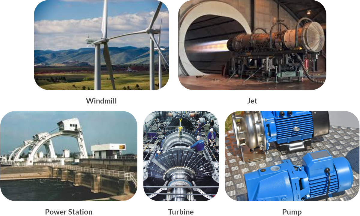
Fig. 3.1 Examples of process equipment used in industry.

In this chapter you will become acquainted with the principles of fluid mechanics, namely with the different types of flow, the Bernoulli law and pressure losses in pipes.

3.2. Fluids in motion

3.2.1. Different types of flow

Flows in a gas or in a liquid are often described with the help of streamlines. Streamlines show how the gas or liquid particles move. Now consider the flow through a pipe section. If we neglect friction, the speed of all particles on line \(I\) (perpendicular to the streamline) is the same. We call this flow laminar frictionless flow (Fig. 3.2(a)).

Note

In English, the flowing medium is referred to as fluid, regardless of whether it is a gas or a liquid.

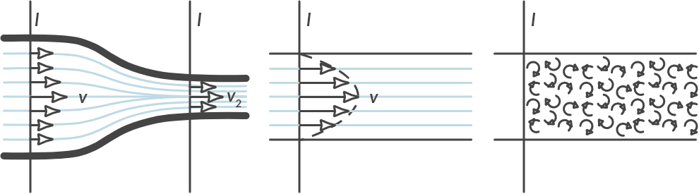
Fig. 3.2 (a) laminar frictionless, (b) laminar, (c) turbulent flow.

When we consider friction, the situation changes. The velocity of the particles on the wall of the pipe is zero and maximum in the middle. In a pipe with a circular cross-section, the velocity runs parabolic from the center with radius \(r\) We call this flow laminar flow (Fig. 3.2(b)).

If the velocity of the fluid becomes too high, the fluid elements no longer follow a straight line. Vortices and fluctuations of the flow over time arise. There is turbulent flow, something you also notice in an airplane.

3.2.2. Viscosity

In reality there is always friction. The more viscous the liquid, the more friction. The viscosity \(\eta\) of a liquid is a measure of the resistance that a liquid gives to movement. In Fig. 3.3 you can see two parallel plates, the upper one moving at a speed \(v\) and the lower one being stationary. There is a liquid between the plates. Because the liquid with viscosity \(\eta\) is viscous, a force \(F\) is required to move the upper plate at a constant speed.

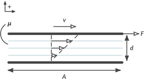
Fig. 3.3 Shear flow in a rheometer to measure viscosity \(\eta\).

The force \(F\) required depends on the size of the contact surface \(A\), the speed \(v\) of the upper plate, the viscosity \(\eta\) of the liquid and the thickness \(d\) of the liquid layer. As long as the liquid flow is laminar, the following applies:

(3.1)\[F=\frac{\eta Av}{d}\]

With, \(F\) the necessary force in \([\textrm{N}]\), \(A\) the contact surface in \([\textrm{m}^2]\), \(v\) the velocity of the upper plate [m/s], \(d\) the thickness of the fluid layer in [m] and \(\eta\) the viscosity of the liquid in [Pa·s].

The velocity of the liquid at the upper plate is \(v\), on the lower plate the liquid is stationary. The derivative of speed \(v\) to the position \(y\) is also referred to as the velocity-gradient.

If the ratio between the force \(F\) and \( \displaystyle \frac{v}{d}\) is constant for any \(v\) or \(d\), then we speak of Newtonian behavior and the viscosity \(\eta\) is constant. This is almost always assumed unless we are dealing with complex liquids. Unlike simple fluids that follow Newton’s law of viscosity (where the viscosity is constant regardless of the applied shear rate), complex fluids often exhibit non-Newtonian behavior. This means their viscosity can change depending on the rate of deformation or stress applied to them:

• Shear-Thinning: Viscosity decreases with increasing shear rate (e.g., ketchup, paint).

• Shear-Thickening: Viscosity increases with increasing shear rate (e.g., cornstarch in water, certain polymers).

• Thixotropy: Viscosity decreases over time under constant shear, and recovers when the shear is removed.

Complex fluids also can exhibit both viscous (fluid-like) and elastic (solid-like) responses. This is called viscoelasticity. When subjected to stress, they may temporarily deform and then return to their original shape, similar to how a rubber band behaves.

3.2.3. Continuity equation

The mass flow \(\dot{m}\) is the mass of water that passes through a cross section per second.

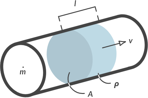
Fig. 3.4 Mass that crosses a section per second.

The following applies to the mass flow:

(3.2)\[ṁ = \frac{∂m}{∂t} = ρ\frac{∂V}{∂t} = ρ\frac{∂(l \cdot A)}{∂t} = ρ(A\frac{∂l}{∂t} + l\frac{∂A}{∂t}) = ρA\frac{∂l}{∂t} = ρAv\]

In which \(\dot{m}\) (pronounced “m-dot” or fluxie m) is the mass flow in [kg/s], \(\rho\) the density of the flowing medium in \([\textrm{kg/m}^3]\), \(A\) is the cross-section of the pipe in \([\textrm{m}^2]\) and \(v\) the flow speed in [m/s]. It is assumed that \(\rho\) (incompressible, therefore non-compressible, liquid) and \(A\) (non-deformable pipe) are constant. The volume flow \(\Phi_v = A \cdot v\) \([m^3/s]\) indicates the displaced volume of liquid.

If we define a control volume in a liquid, the principle of preservation of mass applies to that control volume: no mass accumulates, and no mass disappears. This means that the mass inflow must be equal to the mass outflow.

T-piece

Below you can see the top view of a horizontally located T-piece. Determine the outgoing flow rates as a function of the incoming flow rates: Given: \(A_2 = A_3 = 0.5 \cdot A_1\)

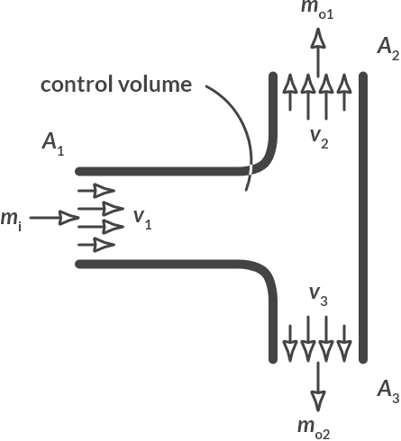
Fig. 3.5 T-piece with incoming and outgoing mass flows.

From conservation of mass, with i=in and o=out follows:

(3.3)\[ \begin{align}\begin{aligned}\begin{split} \dot{m}_i = \dot{m}_{o1} + \dot{m}_{o2}\\\end{split}\\\begin{split}\left.\begin{aligned} \rho A_1 v_1 = \rho A_2 v_2 + \rho A_3 v_3 \\ A_2 = A_3 = 0.5A_1 \end{aligned}\right\rbrace A_1 v_1 &= 0.5A_1 v_2 + 0.5 A_1 v_3 \\ v_1 &= 0.5 v_2 + 0.5 v_3\end{split}\end{aligned}\end{align} \]

If we assume for this equation that \(v_2 = v_3\) then \(v_2 = v_3 = v_1\).

3.2.4. Bernoulli’s prinicple

If you open the door in a flying plane, you will be sucked outside. If you blow past a sheet of paper, the sheet moves to the side you are blowing past (try it!). These phenomena can be explained by Bernoulli’s principle.

Daniel Bernoulli (1700-1782) [1]

Daniel Bernoulli (8 February [O.S. 29 January] 1700 – 27 March 1782) was a Swiss mathematician and physicist and was one of the many prominent mathematicians in the Bernoulli family from Basel. He is particularly remembered for his applications of mathematics to mechanics, especially fluid mechanics, and for his pioneering work in probability and statistics. His name is commemorated in the Bernoulli’s principle, a particular example of the conservation of energy, which describes the mathematics of the mechanism underlying the operation of two important technologies of the 20th century: the carburetor and the aeroplane wing.

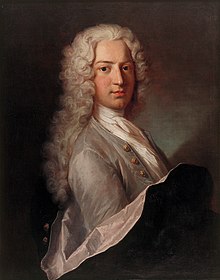
Fig. 3.6 Portrait of Daniel Bernoulli (c. 1720-1725).

When a liquid is at rest, the hydrostatic pressure \(p\) is determined by the height of the liquid column. When the fluid is in motion, there is also dynamic pressure. Bernoulli’s principle describes how the pressure that a liquid exerts on its environment not only depends on the height of the liquid, but also on the velocity of the flow.

Bernoulli’s principle can be derived by applying the law of conservation of energy (\(\Delta W = \text{ potential energy } \Delta E_p + \text{ kinetic energy } \Delta E_k\)) to a mass element in the liquid. You do not need to be able to reproduce this derivation within the framework of this course. It is advisable to study this for understanding.

A mass element in a stationary flow moves over a streamline. We look at one such mass element at two moments, at \(t = t_0\) and at \(t = t_0 + \Delta t\). The velocity of the mass particle increases because the cross section decreases (continuity equation). This change in velocity is also related to a pressure difference.

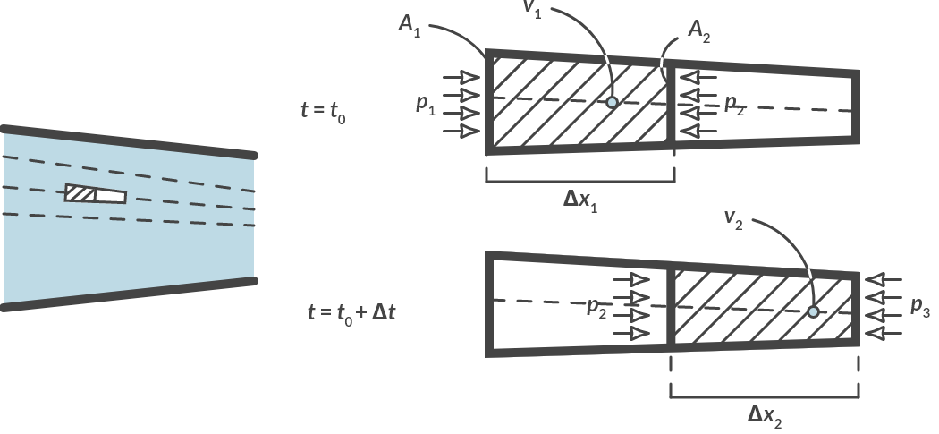
Fig. 3.7 (a) Top view of horizontal flow with increasing speed, (b) mass particle considered in detail.

Applying the law of conservation of energy to a horizontal flow with increasing velocity as in Fig. 3.7 gives:

(3.4)\[\begin{split}W = \Delta E_k \ (\text{since} \ \Delta E_p = 0) \\ W_{p1} - W_{p2} = \frac{1}{2} m v^{2}_{2}-\frac{1}{2}mv^{2}_{1}\end{split}\]

The change in velocity of the mass particle is also accompanied by a change in shape of the mass particle. Its diameter becomes smaller, and its length becomes larger, but its mass remains the same. If its density remains the same (and we assume that for liquids), its volume will remain the same. For the volumes we can write:

(3.5)\[V_1 = A_1 \Delta X_1; \ V_2 = A_2 \Delta X_2; \ V_1 = V_2 = V\]

The work of the pressure equals the force times the distance traveled. At \(t = t_0\) a pressure \(p_1\) acts on the left side of the mass particle and a pressure \(p_2\) on the right side. At \(t = t_0 + \Delta t\) there is pressure \(p_2\) on the left of the particle and \(p_3\) on the right. We assume that the pressure difference over the particle remains constant for a while. (For a small displacement that is allowed.)

The conservation of energy from (3.4) then becomes:

(3.6)\[\begin{split}F_{p1} \Delta X_{1} - F_{p2} \Delta X_{2} = \frac{1}{2} m v^{2}_{2} - \frac{1}{2} m v^{2}_{1} \\ p_{1} A_{1} \Delta X_{1} - p{2} A_{2} \Delta X_{2} = \frac{1}{2} m v^{2}_{2} - \frac{1}{2} m v^{2}_{1}\end{split}\]

With equation (3.5) and by dividing left and right by \(v\) we finally get:

(3.7)\[\begin{split}p_{1} A_{1} \Delta X_{1} - p_{2} A_{2} \Delta X_{2} = \frac{1}{2} ρ V v^{2}_{2} - \frac{1}{2} ρ V v^{2}_{1} \\ \frac{p_{1} A_{1} \Delta X_{1}}{V} - \frac{_{2} A_{2} \Delta X_{2}}{V} = \frac{1}{2} ρ v^{2}_{2} - \frac{1}{2} ρ v^{2}_{1}\end{split}\]

(3.8)\[\frac{p_{1} A_{1} \Delta X_{1}}{A_1 \Delta X_1} - \frac{_{2} A_{2} \Delta X_{2}}{A_2 \Delta X_2} = \frac{1}{2} ρ v^{2}_{2} - \frac{1}{2} ρ v^{2}_{1}\]

(3.9)\[p_1 + \frac{1}{2} ρ v^{2}_{1} = p_2 + \frac{1}{2} ρ v^{2}_{2}\quad \quad [Pa] = [kgm^{-3}][m^{2}s^{-2}]\]

Equation (3.9) is Bernoulli’s principle, if there is no difference in height in the flow. To now also take into account the effect of height differences, we do the same derivation for a vertical flow.

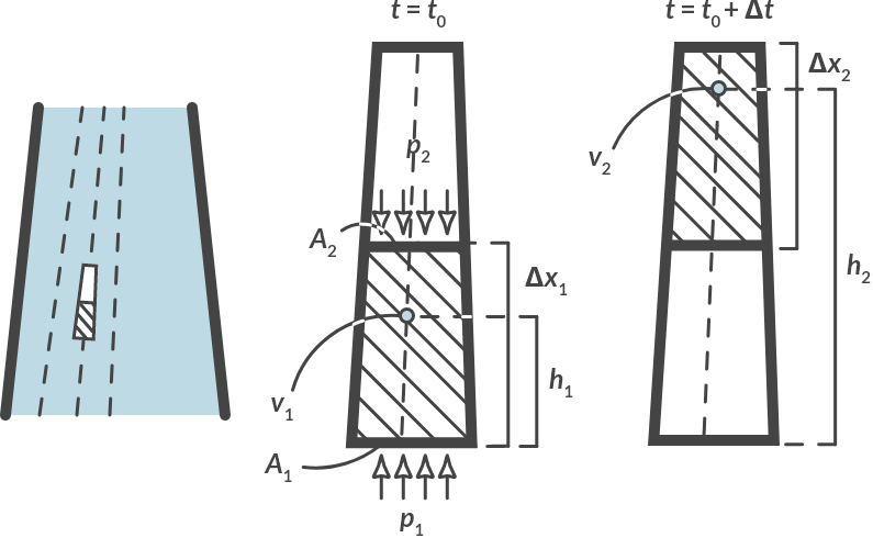
Fig. 3.8 (a) Front view of a vertical flow with increasing speed, (b) mass particle considered in detail.

In addition to a change in kinetic energy, a change in potential energy also plays a role. Applying the conservation of energy now gives:

(3.10)\[\begin{split}w = \Delta E_k + \Delta E_p \\ W_{p1} - W_{p2} = \frac{1}{2} m v^2_2 - \frac{1}{2}mv^2_1 + m g h_2 - m g h_1\end{split}\]

With equation (9.4) and by dividing left and right by \(v\) we finally get:

(3.11)\[p_{1} + \frac{1}{2} ρ v^{2}_{1} + ρ g h_1 = p_2 + \frac{1}{2} ρ v^{2}_{2} + ρ g h_2\]

Or

(3.12)\[p_1+\frac{1}{2} ρ v^{2}_{1} + ρ g h_1 = \textrm{constant}\]

on one streamline.

All terms have the unit \([Nm^{-2}] = \textrm{[Pa]}\).

The term \(p\) is the static pressure relative to the environment (pump, air pressure and liquid column pressure).

The terms \(\rho gh\) represent the potential energy of a liquid at height \(h\).

Pay attention! this is not the height of the liquid column, but the height of the streamline.

The term \(\frac{1}{2} ρ v^2\) expresses the kinetic energy of a fluid with a speed \(v\). This term is also called the dynamic pressure.

This is the complete principle of Bernoulli. Which only applies to one streamline within stationary flow.

Draining barrel

With which velocity does the barrel drain?

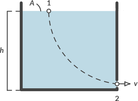
Fig. 3.9 Draining barrel.

We choose the points 1 and 2 on a streamline. The following applies

• \(p_1 = p_2 = p_{\text{atmosphere}}\)

• \(h_1 = h, h_2 = 0\)

• \(v_1 ≈ 0, v_2 = v\)

Applying the Bernoulli law gives:

(3.13)\[\begin{split} p_1 + ρ g h_1 + \frac{1}{2} ρ V^{2}_{1} = p_2 + ρ g h_2 + \frac{1}{2} ρ V^{2}_{2} \\ ρ g h_1 = \frac{1}{2} ρ V^{2}_{2} \to V_2 = \sqrt{2gh_1} \end{split}\]

Note

With a frictionless free fall from height \(h\) of a mass \(m\), the same relationship applies. Try to deduce this. Note that the size of the falling mass does not play a role in the value of that final velocity.

Pipe with height difference

How much force is needed to operate a sprinkler system at a height of 4 meters at a speed of 5 \([\textrm{m/s}]\)? Use \(A_1 = 100\ [\textrm{mm}^2], A_2 = 1\ [\textrm{mm}^2]\).

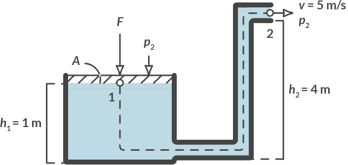
Fig. 3.10 Sprinkler system.

Solution

We choose points 1 and 2 on a streamline. If the outflow opening is small enough, a mass particle at point 1 must pass point 2. The following applies:

• \(p_1 = F/A + p_{\text{atmosphere}}, p_2 = p_{\text{atmosphere}}\)

• \(h_1 = 1\ [\textrm{m}], h_2 = 4\ [\textrm{m}]\)

• \(v_2 = 5\ [\textrm{m/s}], v_1 = \dfrac{v_2 A_2}{A_1} = 0.05\ [\textrm{m/s}]\) as result of continuity equation

Applying Bernoulli’s principle gives:

(3.14)\[\begin{split} p_1 = \rho g h_1 + \frac{1}{2} \rho v_1^2 = p_2 + \rho g h_2 + \frac{1}{2} \rho v_2^2 \\ p_b + F/A = p_b + \rho g (h_2 - h) + \frac{1}{2} \rho (v_2^2 - v_1^2) \\ F/A = 1000 \cdot 9.81 \cdot (4-1) + \frac{1}{2} \cdot 1000 \cdot (5^2 - 0.05^2) \\ F/A = 41.9\ [\textrm{kPA}] \\ F = 4.19\ [\textrm{N}]\end{split}\]

Context: a weight of 0.43 kg on a 1 \(\times\) 1 cm piston can pump water up 3 meters an realize a speed of 5 m/s trough a pipe of 1 \(\times\) 1 mm, at least if there is no friction in the pipe.

Pipe with height difference (continued)

It is insightful to choose some other points on the streamline of points 1 and 2. Below you see points 3 and 4 on the same streamline.

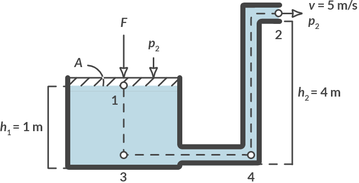
Fig. 3.11 Different points on the same streamline.

For points 1, 2, 3 and 4 the following applies (with \(\frac{F}{A} = 4,19 \cdot 103 \textrm{ [Pa]}\)):

	In point 1	In point 3	In point 4	In point 2
\(p\)	\( F/A + p_b\)	\( F/A + p_b + \rho g \cdot 1\)	\( p_b + \rho g \cdot 4\)	\( p_b\)
\(\rho g h\)	\( \rho g \cdot 1\)	\( 0 \)	\( 0 \)	\( \rho g \cdot 5\)
\(0.5 \rho V^2 \)	\( 0.5 \rho \cdot 0.05^2\)	\( 0.5 \rho \cdot 0.05^2\)	\( 0.5 \rho \cdot 5^2\)	\( 0.5 \rho \cdot 5^2\)
\(\Sigma\)	\( p_b + 51.74\ [\textrm{kPA}]\)	\( p_b + 51.74\ [\textrm{kPA}]\)	\( p_b + 51.74\ [\textrm{kPA}]\)	\( p_b + 51.74\ [\textrm{kPA}]\)

You see that the sum of the three terms (static pressure, potential energy and kinetic energy per volume element) is the same in every point! It is advisable though to choose your points smartly (point 4 is not such an easy choice!).

3.3. Pressure loss in pipes

We have already seen in Section 3.2 that flowing fluid experiences a frictional force. If we pump a liquid through a pipe, an extra pressure is needed to overcome this wall friction. We say that the frictional force leads to a pressure loss in the pipe. The pressure loss due to wall friction is generally dependent on three factors:

• the liquid velocity (and therefore the flow rate and the diameter of the pipe),

• the surface condition (roughness) of the inner wall and

• the fluid properties such as the density and viscosity of the fluid.

It is common to relate the pressure drop to the average velocity \(v\) of the flow with the Darcy friction factor \(f\):

(3.15)\[\Delta p_{\textrm{loss}} = f \frac{L}{D} \frac{1}{2} ρ v^2\]

with:

• \(\Delta p\) the pressure loss in the pipe in [Pa],

• \(L\) the length of the pipe in [m],

• \(D\) the diameter of the pipe in [m],

• \(\eta\) the density of the liquid in \([kg/m^3]\),

• \(v\) the average (bulk) speed of the flow in [m/s] and

• \(f\) de Darcy friction factor [-].

Henry Darcy (1803 - 1858) [2]

Henry Philibert Gaspard Darcy (10 June 1803 – 3 January 1858) was a French engineer who made several important contributions to hydraulics, including Darcy’s law for flow in porous media.

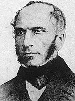
Fig. 3.12 Portrait of Henry Darcy.

In a laminar flow the frictional force (and therefore the pressure loss) can be deduced from (3.1).

This derivation lies outside the scope of this course.

The following applies to the pressure loss with laminar flow:

(3.16)\[ \Delta p_{\text{loss}} = f \frac{L}{D} \frac{1}{2} ρ v^2; \quad f=\frac{64}{R_e}; \quad R_e = \frac{ρ v D}{\eta}.\]

In this equation, the dimensionless Reynolds number Re indicates the ratio between the inertial forces (\(\propto \rho\)) and the resistance forces (\(\propto \eta\)). The flow is laminar if the Reynolds number is less than 2100. For a laminar flow the friction factor is a simple function of the Reynolds number, namely \(f = \frac{64}{Re}\). The pressure drop is linear depending on the velocity and the power required to move the liquid is equal to the product of the pressure drop and volume flow.

With increasing Reynolds number, it appears that the flow is changing from laminar to turbulent. In a laminar flow, the speed at a certain position is always the same, which also means that particles released at a certain position always follow the same path. These properties are not retained if the flow becomes turbulent. The current develops a very random movement with rapid irregular movements in both time and space. These irregularities occur spontaneously, although the imposed conditions are kept the same.

As a result, the relationship between the friction and the average speed in a turbulent flow is not clear. Therefore, the coefficient of friction can only be determined empirically or via numerical methods.

The results of the experiments are recorded in the Moody diagrams, named after the first diligent worker who compiled the enormous amount of data in 1944 into a more convenient format. These diagrams show the friction factor as a function of the Reynolds number. A simplified Moody diagram is shown in Fig. 3.11.

For incompressible media, the losses due to friction are traditionally included in the pipeline as an additional pressure term in the Bernoulli equation.

(3.17)\[ p_1 + ρ g h_1 + \frac{1}{2} ρ v^2_1 - \Delta p_{\textrm{loss}} = p_2 + ρ g h_2 + \frac{1}{2} ρ v^2_2\]

The term \(\Delta p_{\textrm{loss}}\) indicates that in point 2 the total energy (per volume element) of the flow (sum of stationary pressure (\(p_2\)), the potential energy (\(\rho g h_2\)) and the kinetic energy (\(\frac{1}{2} \rho V^2\))) is equal to the total energy in point 1 minus the pressure loss.

History

People have been using pipelines for centuries. Clay pipes were found in the ruins of Babylon; During excavations in Pompeii, a lead water pipe system, complete with bronze plug valves, was found. Until the 1900s, wooden pipes were used for certain applications. After having understood how cannons were to be cast in the 15th century, they also started to cast iron pipes. Cast iron pipes are still used, mainly for sewage systems. With the invention of the steam engine in the 18th century, demand also came for pipes that can withstand high pressure and higher temperatures. Steel tubes were made by coiling a steel band and then forgin them together. After the first world war it became possible to make seamless pipes, which gave a major boost to the development of process and energy companies. Although more steel than cast iron pipes have been made since the 19th century, the housings of valves and fittings are still casted. Even today, this is often the cheapest method. The development of mobile welding equipment made it possible to make long pipes. Initially, acetlylene-oxygen burners were used for this, but arc welding has been on the rise in recent years.

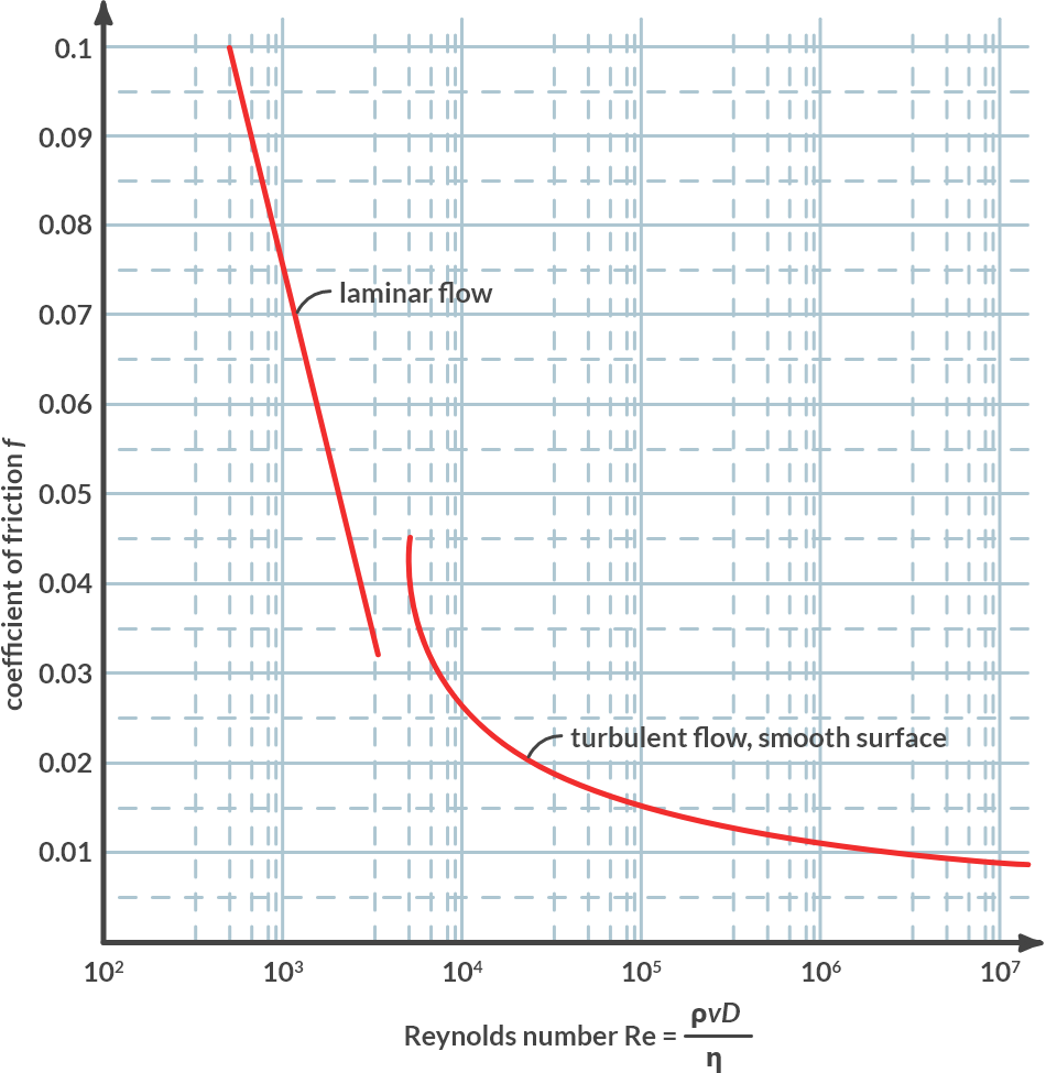
Fig. 3.13 Moody diagram.

Pipe with height difference (continued)

In Example 3 the friction in the pipe is neglected. We assume that the total length of the pipe is 6 m and that the diameter of the pipe is 1.1 mm (which corresponds to an outflow area of 1 mm\(^2\)). Given is the density of water \(\rho = 1000\ [\textrm{kg/m}^3]\), and the dynamic viscosity of water, \(\eta = 1 \cdot 10^{-3}\ [\textrm{Ns/m}^2]\). Then calculate the force that is required to achieve the desired spray rate.

To determine whether the flow is turbulent or laminar, we first determine the Reynolds number:

(3.18)\[ R_e = \frac{\rho v D}{\eta} = \frac{1000 \cdot 5 \cdot 1.1 \cdot 10^{-3}}{1 \cdot 10^{-3}} = 5.5 \cdot 10^3 \]

The flow is turbulent (Re > 2100). From Fig. 3.11 we can see that the friction factor \(f\) is approximately 0.044. Instead of expression (3.14) we can then write:

(3.19)\[\begin{split} p_1 + \rho g h_1 + \frac{1}{2} \rho v^2_1 = p_2 + \rho g h_2 + \frac{1}{2} \rho v^2_2 + \Delta p_{\textrm{loss}} \\ p_b + \frac{F}{A} = p_b + \rho g (h_2 - h_1) + \frac{1}{2} \rho (v^2_2 - v^2_1) + f \frac{L}{D} \frac{1}{2} \rho v^2_2 \\ \frac{F}{A} = 1000 \cdot 9.81 \cdot (4-1) + \frac{1}{2} \cdot 1000 \cdot (5^2-0.05^2) + 0.044 \cdot \frac{6}{1.1 \cdot 10 ^{-3}} \frac{1}{2} \cdot 1000 \cdot 5^2 \\ \frac{F}{A} = 419 \cdot 10^3 + 3.0 \cdot 10^6 \quad \textrm{[Pa]} \\ F = 3.0 \cdot 10^3 \quad \textrm{[N]}\end{split}\]

That makes quite a difference with the original outcome! By far the largest part of the force is needed to overcome the wall friction losses.

Hydroelectric station

Using the Bernoulli equation, we can also estimate how much power the hydroelectric station in the Hoover dam can generate (Fig. 3.13 a and b).

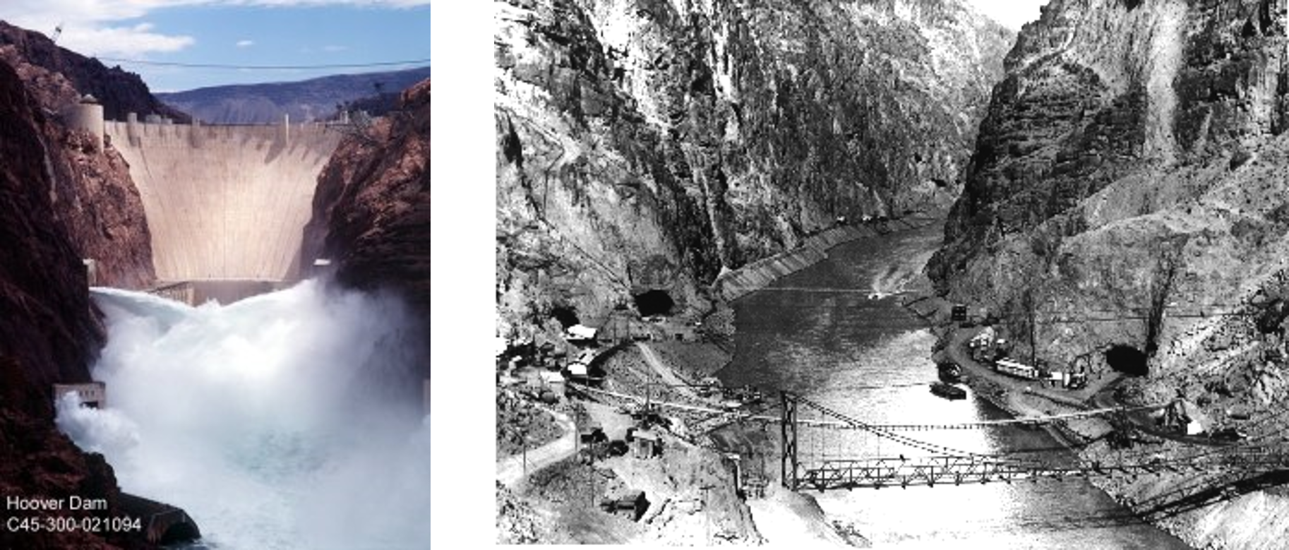
Fig. 3.14 (a) De hydroelectric station in the Hoover dam, (b) the canyon before the construction of the hydroelectric plant.

The starting point for our estimate is the diagram from Fig. 3.13 of the plant. The water first falls over a height of 180 m. After arriving at the bottom it flows through 4 pipes, each 358 m long. Then each line divides into four. The 16 lines of 110 m eventually lead to so-called Francis turbines, which convert the movement of the water into rotational energy, which is converted into electricity by generators.

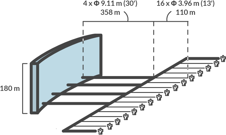
Fig. 3.15 Schematic of the Hoover dam installation.

Furthermore, it is known (from the website) that the total volume flow through the power station can be up to \(\phi_{V,tot} = 1274\ [\textrm{m}^3/\textrm{s}]\).

1. Calculate the total pressure loss of the running water over the pipes that run from the Hoover dam to the turbines.

Solution

1. The volume flow through each of the four supply lines is \(\phi_{V1} = 1274/4 = 319\ [\textrm{m}^3/\textrm{s}]\)

The flow-through area of the first pipes is equal to: \(A_1 = \pi D^2/4 = 4(9.11)^2/\pi = 65.2\ [\textrm{m}^2]\).

The average velocity in this section \(v_1 = \phi_{V1}/A_1 = 319/65.2 = 4.9 \textrm{ [m/s]}\).

The Reynolds number becomes:

(3.20)\[ R_e = \frac{\rho v D}{\eta} = \frac{1000 \cdot 4.9 \cdot 9.11}{10^{-3}} = 4.4 \cdot 10^7 \]

We are thus on the far right of Fig. 3.11 (turbulent); the friction factor is then almost constant with a value of 0.008. The pressure loss over these pipes becomes:

(3.21)\[ \Delta p = f \frac{L}{D} \frac{1}{2} \rho V^2 = 0.008 \frac{358}{9.11} \frac{1}{2} 1000 \cdot (4.9)^2 = 3.7 \cdot 10^3 \quad \textrm{[Pa]} \]

This same approach can be used for the thinner pipes to the turbines:

(3.22)\[ V_2 = \frac{\varphi_{V2}}{A_2} = \frac{\frac{\varphi_{V,tot}}{16}}{\frac{1}{4} \pi D^2_2} = \frac{1274}{4 \pi \cdot 3.96^2} = 6.5 \quad \textrm{[m/s]} \]

(3.23)\[ R_e \frac{\rho v D}{\eta} = \frac{1000 \cdot 6.5 \cdot 3.96}{10^{-4}} = 6.6 \cdot 10^8 \to f = 0.008\]

(3.24)\[ \Delta p = f \frac{L}{D} \frac{1}{2} \rho V^2 = 0.008 \frac{110}{3.96}\frac{1}{2} 1000 \cdot (6.5)^2 = 4.7 \cdot 10^3 \quad \textrm{[Pa]} \]

The total pressure loss over the pipes thus becomes \((3.7 + 4.7) \cdot 10^3 = 8.4 \cdot 10^3 \quad \textrm{[Pa]} (= 0.084 \textrm{ [bar]})\) per streamline.

2. Calculate the dynamic pressure available for the turbines. Calculate the power that the station can deliver. The hydrodynamic power can be calculated with \(P = \Delta p \cdot \phi_V\).

Solution

2. The figure below shows a streamline that runs from the lake at the top of the Hoover dam, to the turbine in the power station:

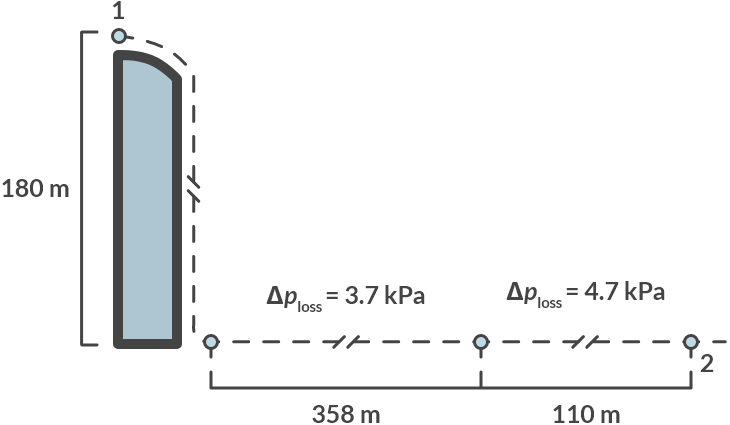
Fig. 3.16 Streamline from the Hoover dam to the turbine.

We define points 1 and 2 on the streamline:

For point 1 we assume that \(p_1 = p_{\textrm{atmosphere}}, v_1 = 0 \quad \textrm{[m/s]}\) and \(h_1 = 180 \textrm{ [m]}\).

For point 2 we assume that \(p_2 = p_{\textrm{atmosphere}}, v_2 = v \quad \textrm{[m/s]}\) and \(h_1 = 0 \textrm{ [m]}\).

We also include the pressure losses that we have calculated under a.

(3.25)\[\begin{split} p_1 = \rho g h_1 + \frac{1}{2} \rho v^2_1 - \Delta p_{\textrm{loss}} = p_2 + \rho g h_2 + \frac{1}{2} \rho v^2_2 \\ p_{atm} + \rho g h_1 + \frac{1}{2} \rho v (0)^2 - \Delta p_{\textrm{loss}} = p_{\textrm{atm}} + \rho g 0 + \frac{1}{2} \rho v^2_2 \\ \frac{1}{2} \rho v^2_2 = \rho g h_1 - \Delta p_{\textrm{loss}} = 1000 \cdot 10 \cdot 180 - 8.4 \cdot 10^3 = 1.8 \cdot 10^6 \textrm{ [Pa]} \end{split}\]

Assuming that this dynamic pressure of \(1.8 \cdot 10^6 \quad \textrm{[Pa]}\) is fully converted into electricity; the plant can deliver: \(P = \Delta p \phi_V = 1.8 \cdot 10^6 \cdot 1274 = 2.29 \quad \textrm{[GW]}\).

3. How much power is lost to friction? Calculate the efficiency.

Solution

Friction causes a pressure loss of \(8.4 \cdot 10^3 \textrm{ [Pa]}\). This means that friction in the pipes \(P = \Delta p \cdot \phi_V = 8400 \times 1274 = 10.7 \textrm{ [MW]}\) of frictional heat. The efficiency in the transport system is then (\(2.29 \cdot 10^9 – 10.7 \cdot 10^6) / 2.29 \cdot 10^9 = 0.995 = 99.5 \%\).

Note

Due to the numerical values of the Moody diagram, it is not possible to work parametrically here.

3.4. Fluid machines

Due to flow losses, the pressure in a flowing medium slowly decreases, but the pressure can also be increased by adding energy. You can add energy to a flow, for example with a pump or a compressor. Due to the rotating movement of the pump, liquid is propelled and there is an increase in pressure over the pump. The added pressure through the pump is then \(\Delta p_{\textrm{pump}} = p_3 - p_4\) in which \(p_3\) is the pressure after the pump and \(p_4\) before the pump. The energy conservation comparison of a piping system with a flow machine is then equal to (3.17), the term \(\Delta p_{\textrm{pump}}\) then being added as a positive term on the left-hand side. The power that is added to the flow is then equal to \(P = \Delta p \cdot \Phi_v\) where \(\Phi_v\) is the volume flow that is shifted by the pump. In this way, mechanical energy from the pump (or ultimately perhaps electrical energy if it concerns an electric pump) becomes potential energy from the flow. The mechanical (or electrical) power that the pump uses is usually significantly larger than the power \(P = \Delta p \cdot \Phi_v\) absorbed by the flow. This is due to losses, so that the efficiency of the pump is less than 100%. The impeller of the pump also creates swirls and turbulence that are eventually dissipated and transferred to heat (that heat increase is usually small). Designing the correct geometry of a pump is therefore very important and a subject that plays an important role in mechanical engineering.

Not only can energy be added to a flow, energy can also be extracted, as can be seen for example in Fig. 3.8 of the hydroelectric station. Energy is often extracted by a fan that is driven by the current, such as a windmill or a turbine. A turbine is similar to a pump, but the energy is now added to the flow. Now a pressure loss term must be added to (3.17) as a loss term so the term \(- \Delta p_{\textrm{turbine}}\) is added to the left-hand side.

Note

The minus sign indicates that energy is extracted. The design of the correct form of blades for a windmill or a turbine is also an important subject in mechanical engineering.

3.5. To be continued

What lies ahead

In this chapter you have become acquainted with the fields of liquids and flow. The theory in the field of flow can still be considerably expanded. In fact, the theory needs to be expanded further because a turbulent flow is still not fully understood. Einstein called this the last unsolved problem in physics.

For the design process of these devices, it is necessary to have insight into both the small-scale physical phenomena that play a role and the relationship between the device and the other parts of the installation. Flow analysis leans against the field of physical transport phenomena from physics.

In practice, flow devices for the compression and expansion of liquids and gases are often used in combinations with all kinds of other processes and devices, for example reactors (process devices), combustion for power generation (e.g. in an engine or gas turbine), or phase transitions (e.g. in separation devices). Heat machines, in which the heat is added or extracted from the liquid, are already discussed in the next chapter. In the mechanical engineering curriculum you also receive various follow-up courses that continue with this topic.

---

[1]

https://en.wikipedia.org/wiki/Daniel_Bernoulli

[2]

https://en.wikipedia.org/wiki/Henry_Darcy